read

The Perceptron is a simplest version of Neural network. It is similar to way Logistic regression works.

I already posted about the Logistic regression on my post for Machine learning.

To remind, I will explain more detail of Logistic regression.

This post is based on the video lecture¹

Logistic regression

Logistic regression can be considered as a very tiny Neural network having no hidden layer for Classification.

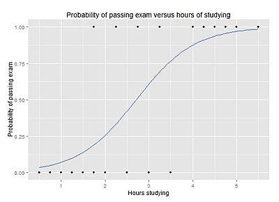
Simply, Logistic regression’s goal is to find a line classifying our input’s labels.

When the input value is smaller than $0.5$, the input value is classified as 0 otherwise 1.

Why the name is logistic?

Look at the graph of logistic function.

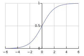
The logistic function make a line curved.

We can define the equation of Logistic regression like the below.

\[\begin{align} & \text{Given $x$, want $\hat{y} = P(y=1 \vert x)$}\\ & \text{input: }X \in R^{n_x} \\ & \text{parameters: } w \in R^{n_x}, b\in R \\ & \text{output: } \hat{y} = \sigma(w^Tx + b)\\ \end{align}\]

The other equation is like the below equation. It is totally same.

\[\begin{align} &X_0 = 1, X \in R^{n_x+1}\\ & \theta = \begin{bmatrix} \theta_0 \\ \theta_1 \\ \vdots \\ \theta_{n_x} \\ \end{bmatrix}, \theta_0 = b\\ & \hat{y} = \sigma(\theta^T x)\\ \end{align}\] \[\hat{y} = \sigma(w^Tx + b), \text{where }\sigma(z) = \frac{1}{1+e^{-z}}\] \[\begin{cases} \text{if $z$ is very large, }\sigma(z) \approx \frac{1}{1+0} = 1\\ \text{else $z$ is very small, }\sigma(z) \approx \frac{1}{1+\infty} = 0\\ \end{cases}\] \[\text{Given }\left\{ \left( x^{(1)}, y^{(1)} \right), \left( x^{(2)}, y^{(2)} \right), \dots ,\left( x^{(m)}, y^{(m)} \right) \right\}, \\ \text{want } \hat{y}^{(i)} \approx y^{(i)}\]

To achieve our goal, we have to define the loss function.

We will use the MSE(Mean square error) as a loss function.

\[L(\hat{y}, y) =MSE(\hat{y}, y) = (\hat{y}^{(i)} - y^{(i)})^2\]

Cost function is defined the sum of loss function.

\[J(w, b) = \frac{1}{m} \sqrt{\sum_{i=1}^m L(\hat{y}^{(i)}, y^{(i)})} = \frac{1}{m} \sqrt{\sum_{i=1}^m(\hat{y}^{(i)} - y^{(i)})^2}\]

Why do we need loss function, even though accuracy looks like more explicit?

The reason is whether or not it can be differentiated.

Back propagation

Why lost function must be differentiated? Because if we just know the accuracy, we don’t know how to update our weight to minimize our model.

For example, when we know our model’s accuracy is 0.76, Is this useful to update our parameter?

But if we know our cost is 100 by the computation of the cost function, $J = w_1^2 + w_2^2$, Then It might have some information to. Let’s see.

drawing the graph for our cost function give us some insight.

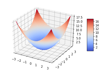
Like the above graph is called as convex function.

The more darker blue, the cost is smaller. So, By moving the parameters($w_1, w_2$) to proper direction, we can get the much smaller cost function.

The direction to move parameters is defined the differentiated parameters. This algorithm is called Gradient descent. It looks like finding the low point by sliding down from the top.

\[w : = w - \alpha \frac{\part J}{\part w}\]

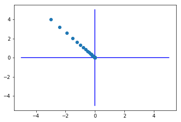
def f(w):
    return w[0]**2 + w[1]**2


init_w = np.array([-3.0, 4.0])
w, history_w = gradient_descent(f,init_w)

plt.plot( [-5, 5], [0,0], '-b')
plt.plot( [0,0], [-5, 5], '-b')
plt.plot(history_w[:,0],history_w[:,1], 'o')
np.arange()
plt.show()

Computation graph

We define logistic regression, and define the cost function.

The purpose of cost function is to find the proper parameters that make cost small with gradient descent.

To update our parameters, we should know $\frac{\part J}{dv}$.

Let’s see the more detail with computation graph.

Assuming that we have a cost function, $J(a,b,c) = 3(a + bc)$.

To get $J$, the equations can be processed like the below,

\[\fbox{u= bc} \to \fbox{v = a + u} \to \fbox{J=3v}\\ u = bc \\ v = a + u\\ J = 3v\]

Chain rule

$\frac{\part J}{dv}$ is can be written as $\frac{\part \text{ FinalOutputVar}}{d\text{ Var}}$ meaning how much affect from input variable to final output variable.

To update our parameters we need to know how much input variables ($b, c$) affect to output.

\[\frac{\part J}{\part b} = \frac{\part J}{\part v} \cdot \frac{\part v}{\part u} \cdot \frac{\part u}{\part b} \\ \frac{\part J}{\part c} = \frac{\part J}{\part v} \cdot \frac{\part v}{\part u} \cdot \frac{\part u}{\part c}\]

It is called as Chain rule that is a formula for computing the derivative of the composition of two or more.

Training Logistic regression

How to train logistic regression?

We can update our weight with Gradient descent and Chain rule.

\[Z = w^T x + b \\ \hat y = a = \sigma(z) \\ L(a, y) = - y \log(a) + (1 - y)\log(1-a)\]

$x$ is input variables, $w$ is weights and $b$ is a bias. Our purpose is to train the model to classify x into labels with weights and bias, $w, b$.

Gradient descent

Gradient descent is used for updating the weights and bias.

\[w : = w - \alpha \frac{\part J}{\part w}\\ b : = b - \alpha \frac{\part J}{\part b}\\\]

Chain Rule

Chain rule is used for calculating the derivative of loss function by weights and bias.

\[\frac{\part L}{\part w} = \frac{\part L}{\part a} \cdot \frac{\part a}{\part z} \cdot \frac{\part z}{\part w} \\ \frac{\part L}{\part b} = \frac{\part L}{\part a} \cdot \frac{\part a}{\part z} \cdot \frac{\part z}{\part b}\]

Cost function

Let’s see the detail of how to define cost function of logistic regression.

\[\begin{align} &\hat y = \sigma (w^T x + b) \text{ where } \sigma(z) = \frac{1}{1 + e^{-z}} \\ \\ & P(y\vert x) =\\ & \hat y ^y (1 - \hat y)^{(1-y)} \begin{cases} &\text{if } y = 1, P(y \vert x) = \hat y ^y( 1 - \hat y)^{(1-y)} = \hat y ^1( 1 - \hat y)^{0} = \hat y \\ &\text{if } y = 0, P(y \vert x) = \hat y^y ( 1 - \hat y)^{(1-y)} = \hat y ^0( 1 - \hat y)^{1}= 1 - \hat y \\ \end{cases} \\ \\ &\log P(y \vert x) = \log (\hat y^y ( 1 - \hat y)^{(1-y)})\\ & =y \log \hat{y} + (1-y) \log (1 - \hat y) \\ & =-L(\hat y, y) \end{align}\]

cost function is defined as the sum of loss function.

• We want to maximize likelihood estimation.
• Minimize the loss corresponds with maximizing $\log P(y \vert x)$.

\[\begin{align} \log P(\text{labels in training set}) =& \log \prod_{i=1}^m P(y^{(i)} \vert x^{(i)}) \\ =& \sum_{i=1}^m \log P(y^{(i)}\vert x^{(i)}) \\ =& -\sum_{i=1}^m L (\hat y^{(i)}, y^{(i)})\\ \\ J(w, b) = - \frac{1}{m} \sum_{i=1}^m L (\hat y^{(i)}, y^{(i)})\\ \end{align}\]

1. https://www.coursera.org/learn/neural-networks-deep-learning?specialization=deep-learning “Deep learning specialization” ↩