In the previous post, the topic is about the how neural networks work. In this post, i will introduce the way to learn the neural network.
In learning process, we will compute the cost function.
Learning Neural Network
There are three ways to develop the algorithms.
- Algorithm by human
- Extracting feature by human’s algorithm, use Machine Learning algorithm.
- Use Deep Learning
Loss function
Loss function is one of index to show the performance of model. The reason why we use loss function instead of using accuracy, loss function is used for fitting the parameter in Back propagation process.
Loss function is useful to get the partial derivative of weight variables.
Mean squared error(MSE)
\[E=\frac{1}{2}\sum_k(y_k - t_k)^2\] \[\begin{align} &\text{If data size is N,}\\ &E = -\frac{1}{2N}\sum_n \sum_k(y_k - t_k)^2 \end{align}\]Cross entropy error(CEE)
\[E = -\sum_k t_k\log y_k\] \[\begin{align} &\text{If data size is N,}\\ &E = -\frac{1}{N}\sum_n\sum_k t_k\log y_k \end{align}\] \[\begin{bmatrix} 1 \\ 0 \\ \vdots \\ 0 \end{bmatrix}^T \times \ \begin{bmatrix} 0.6 \\ 0.01 \\ \vdots \\ 0.4 \end{bmatrix} = -1 \times \log 0.6 = 0.51\]Mini-batch learning
The data size is too big, we can use batch processing. Also, In learning process, we can use batch for learing called mini-batch. To reduce the learning time, we can select random sample from traing data set. Then the seleted random data set will be used for training samples.
Optimization
\[f(x_0,x_1) = x_0^2+x_1^2\]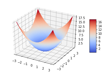
The blue point is small point that has smallest value. We called it as Saddle point
How can we find this point automatically?
Using derivative, you can find the value to be getting close to saddle point
Derivative
\[f'(x)=\lim_{h\rightarrow 0} \frac{f(x+h)-f(x-h)}{2h}\]def numerical_gradient(f,x):
h = 1e-4
grad = np.zeros_like(x)
for idx in range(x.size):
tmp_val = x[idx]
x[idx] = tmp_val + h
fxh1 = f(x)
x[idx] = tmp_val - h
fxh2 = f(x)
grad[idx] = (fxh1 - fxh2) /(2*h)
x[idx] = tmp_val
return grad
Gradient descent
\[x_0 = x_0 - \alpha \frac{\partial f}{\partial x_0}\\ x_1 = x_1 - \alpha \frac{\partial f}{\partial x_1}\\\]def gradient_descent(f,init_x, lr=0.1, step_num=100):
x = init_x
acc_x = list()
for i in range(step_num):
acc_x.append(x.copy())
grad = numerical_gradient(f, x)
x -= lr * grad
return x,np.array(acc_x)
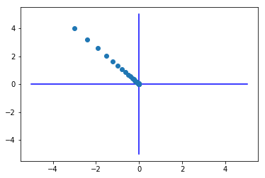
Example
def f(x):
    return x[0]**2 + x[1]**2


init_x = np.array([-3.0, 4.0])
x, history_x = gradient_descent(f,init_x)

plt.plot( [-5, 5], [0,0], '-b')
plt.plot( [0,0], [-5, 5], '-b')
plt.plot(history_x[:,0],history_x[:,1], 'o')
np.arange()
plt.show()
Back propagation
Using the multi layer perception, we can calculate the hypothesis for the XOR problem.
But how can the machine learn the weight and bias from the multilayer?
Here is a solution called back propagation.
The input data affect the result by passing the weights.
Then, using chain rule, the error change the weights by passing from the last layer to first layer.
Partial derivative
Chain rule is $\frac{df(g(x))}{dx}=\frac{df}{dx} = \frac{df}{dg}\cdot\frac{dg}{dx}$
It is basic equation for the partial derivative.
The chain rule is an essential idea for back-propagation.
Softmax with loss computing graph
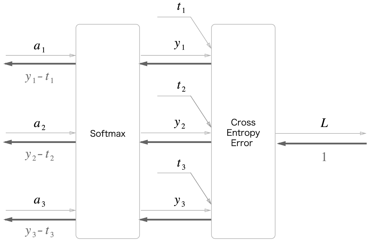
forward calculation
\[\overset{\mathtt{a}}{\longrightarrow} softmax \overset{\mathtt{y_n,\hat y_n}}{\longrightarrow} cross\ entropy \overset{\mathtt{L}}{\longrightarrow}\]Cross entropy : $L(y,\hat{y}) = -\frac{1}{N}\sum_{n \in N}\sum_{i \in N} y_{n,i}log\hat{y}_{n,i}$
Softmax : $y_k = \frac{exp(a_k)}{\sum_{i=1}^n exp(a_i)}$
backward calculation
\[\overset{\mathtt{y_n-t_n}}{\Longleftarrow} softmax \overset{\mathtt{-\frac{t_n}{y_n}}}{\Longleftarrow} cross\ entropy \overset{\mathtt{1}}{\Longleftarrow}\]cost function(loss function)
We will use CEE for cost function.
\(L(y,\hat{y}) = -\frac{1}{N}\sum_{n \in N}\sum_{i \in N} y_{n,i}log\hat{y}_{n,i}\)
We want to find the the value to get derivatie value $\frac{dL}{dx}$ for gradient descent. Using chain rule, we can compute this value easily.
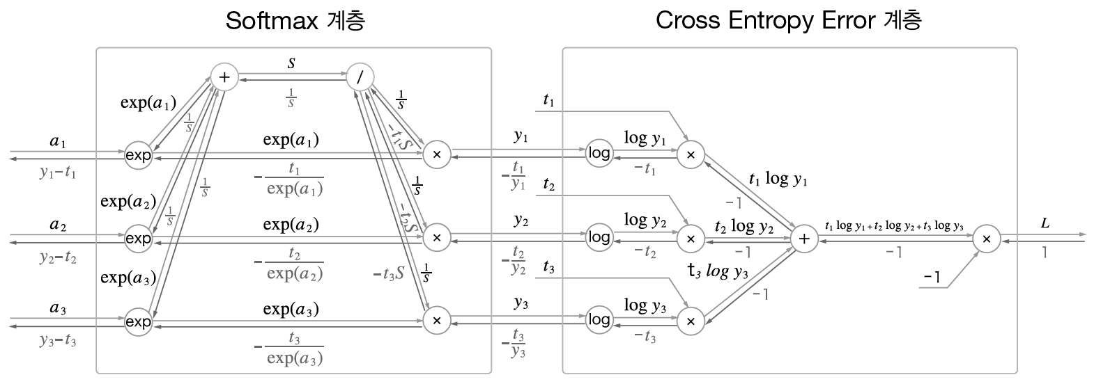
Forward computing graph
\[f_1=\log y_n\\ f_2=t_n \log y_n = t_nf_1\\ f_3=\sum_{k=1}^n t_k \log y_k = \sum_{k=1}^nf_2(y_k)\\ L = f_4 = -\sum_{k=1}^n t_k \log y_k = -f_3\]Backward computing graph
\[\frac{\partial f_1}{\partial y_n} = \frac{1}{y}\\ \frac{\partial f_2}{\partial f_1} = t_n\\ \frac{\partial f_3}{\partial f_2} = \frac{\partial }{\partial f_2(y_n)} \left( f_2(y_1) + \dots + f_2(y_n) \right ) = 1\\ \frac{\partial L}{\partial f_3} = -1\\ \frac{\partial L}{\partial L} =\frac{\partial L}{\partial f_4(y_n)} = 1\\ \frac{\partial L}{\partial y_n} = \frac{\partial L}{\partial f_4} \frac{\partial f_4}{\partial f_3} \frac{\partial f_3}{\partial f_2} \frac{\partial f_2}{\partial f_1} \frac{\partial f_1}{\partial y_n} = 1 \times -1 \times 1 \times t_n \times \frac{1}{y_n} = -\frac{t_n}{y_n}\]To update our weights on the networks, we need to calculate $\frac{dL}{dw}$ how much the value affect the function. Using chain rule of partial derivative, We can derivative $L(y,\hat{y})$ by our weights $W$.
Simple example
\[\begin{align} & z= x\times y\\ & \frac{\partial z}{\partial x} = y\\ & \frac{\partial z}{\partial y} = x\\ \end{align}\] \[\begin{align} z= x + y\\ \frac{\partial z}{\partial x} = 1\\ \frac{\partial z}{\partial y} = 1\\ \end{align}\]import numpy as np
class MulLayer:
def __init__(self):
self.x = None
self.y = None
def forward(self, x, y):
self.x = x
self.y = y
return x*y
def backward(self, dout):
dx = dout * self.y
dy = dout * self.x
return dx, dy
class AddLayer:
def __init__(self):
pass
def forward(self, x, y):
return x+y
def backward(self, dout):
dx = dout * 1
dy = dout * 1
return dx, dy
if __name__=='__main__':
apple = 100
apple_num = 2
orange = 150
oragne_num = 3
tax = 1.1
#layers
mul_apple_layer = MulLayer()
mul_orange_layer = MulLayer()
add_apple_orange_layer = AddLayer()
mul_tax_layer = MulLayer()
#forwad propagation
apple_price = mul_apple_layer.forward(apple, apple_num)
orange_price = mul_orange_layer.forward(orange, oragne_num)
all_price = add_apple_orange_layer.forward(apple_price,orange_price)
price = mul_tax_layer.forward(all_price, tax)
print("Forward| Price:",price)
#Back propagation
dprice = 1
dall_price, dtax = mul_tax_layer.backward(dprice)
dapple_price, dorange_price = add_apple_orange_layer.backward(dall_price)
dapple, dapple_num = mul_apple_layer.backward(dapple_price)
dorange, dorange_num = mul_orange_layer.backward(dorange_price)
print("Backward| apple price:",dapple," apple num:", dapple_num)
print("Backward| orange price:",dorange, " orange num:",dorange_num)
print("Backward| tax:", dtax, " all price:",dall_price)
output
Forward| Price: 715.0000000000001
Backward| apple price: 2.2  apple num: 110.00000000000001
Backward| orange price: 3.3000000000000003  orange num: 165.0
Backward| tax: 650  all price: 1.1
Gradient check
Derivative can be used for checking error of backpropagation. Derivative is easy to make but it is slow comparing to back propagation.
It is obvious that the difference between derivative and backpropagation. If not, it might be error in our codes for back propagation or derviative.
This function is called as Gradient check
The problem in the back propagation
In the case the neural network is deep, the back propagation can’t affect the first weights.
Solution for this problem
Neural networks with many layers really could be trained well, If the weights are initialized in a clever way.
It make rebrand the name to Deep learning
- Our labeled datasets were thousands of times too small.
- Our computers were millions of times too slow.
- We initialized the weights in a stupid way.
- We used the wrong type of non-linearity.